uPDE — you too can solve PDEs

github.com/saadgroup/upde

uPDE

you too can solve PDEs

Describe your PDE the way you write it.
uPDE handles the rest.

uPDE is an expressive Python library designed to solve systems of coupled nonlinear PDEs. It targets physics-focused users — those who want control of their PDE models without worrying about discretization and time integration.

Solve PDEs in 3 Steps

1Define

x = np.linspace(0,1,100)
eq = upde.PDE('u', x)
eq.add_advection(1.0)
eq.add_diffusion(0.01)

2Constrain

def gaussian(x):
  return np.exp(...)
eq.set_ic(gaussian)
eq.set_bc(kind='periodic')

3Solve

sol = eq.solve(
  t_span=(0, 1)
)
# sol.T: (nx, nt)

⏱

Steady & unsteady

Time-marching or direct steady-state with a single switch

Δt

Adaptive timestep

scipy solve_ivp handles step size, error estimation, stiffness

⊞

1D & 2D — same API

Pass y= to go 2D. Code stays identical.

⇌

Coupled systems

PDESystem([eq1, eq2, ...]) with zero boilerplate

∂Ω

Flexible BCs

Dirichlet, Neumann & periodic. One call, any combination.

ƒ

Callable coefs

Spatially- & time-varying. Signature-injected automatically.

Example 01

Nonlinear Diffusion in Porous Media

$$u_t = \left[u^n \, u_x\right]_x$$

1Define

x = np.linspace(0, 1, 200)
eq = PDE('u', x)
eq.add_diffusion(diffusivity=lambda u: u**n)

2Constrain

# compact-support Gaussian IC
u0 = np.exp(-200 * (x - 0.5)**2)
eq.set_ic(u0)
eq.set_bc(kind='dirichlet', side='all', value=0)

3Solve

sol = eq.solve(t_span=(0, 0.1), method='BDF')

plt.plot(x, sol.u[:, 0],  label=f't=0')
plt.plot(x, sol.u[:, -1], label=f't={sol.t[-1]}')

Nonlinear diffusion · BDF solver

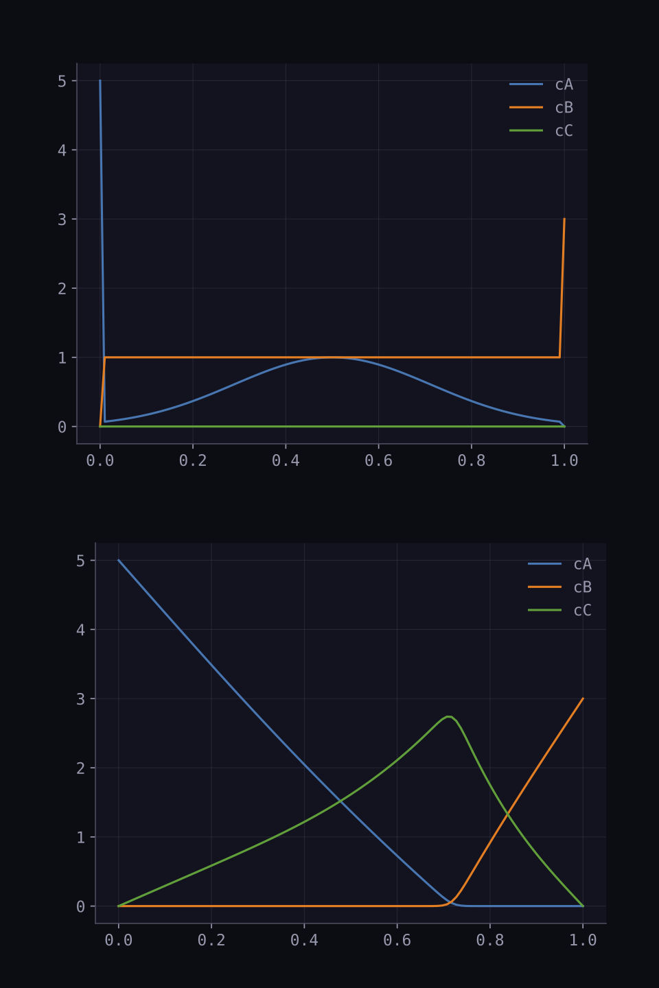
Figure: Porous medium evolution

Replace with your matplotlib output

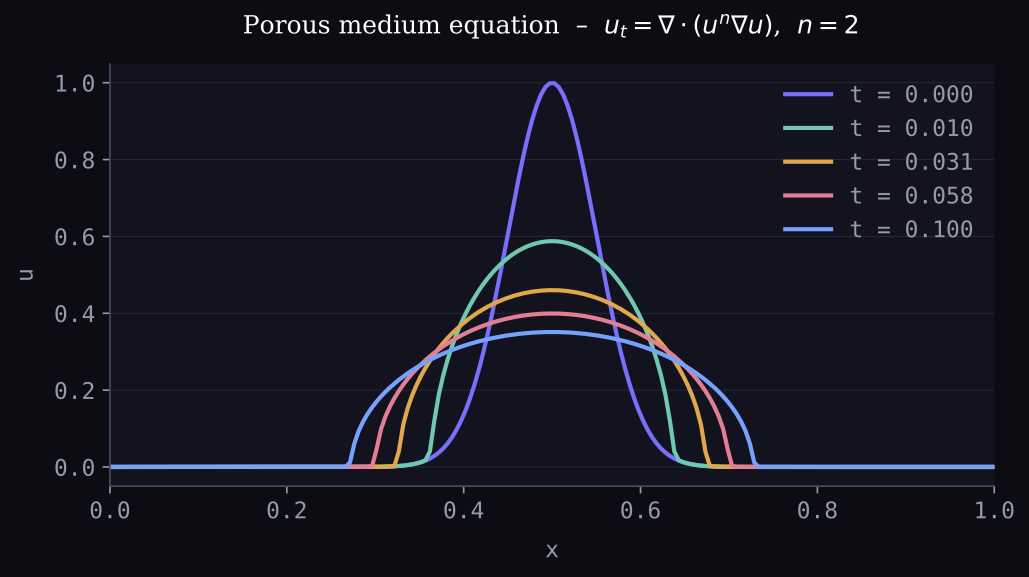
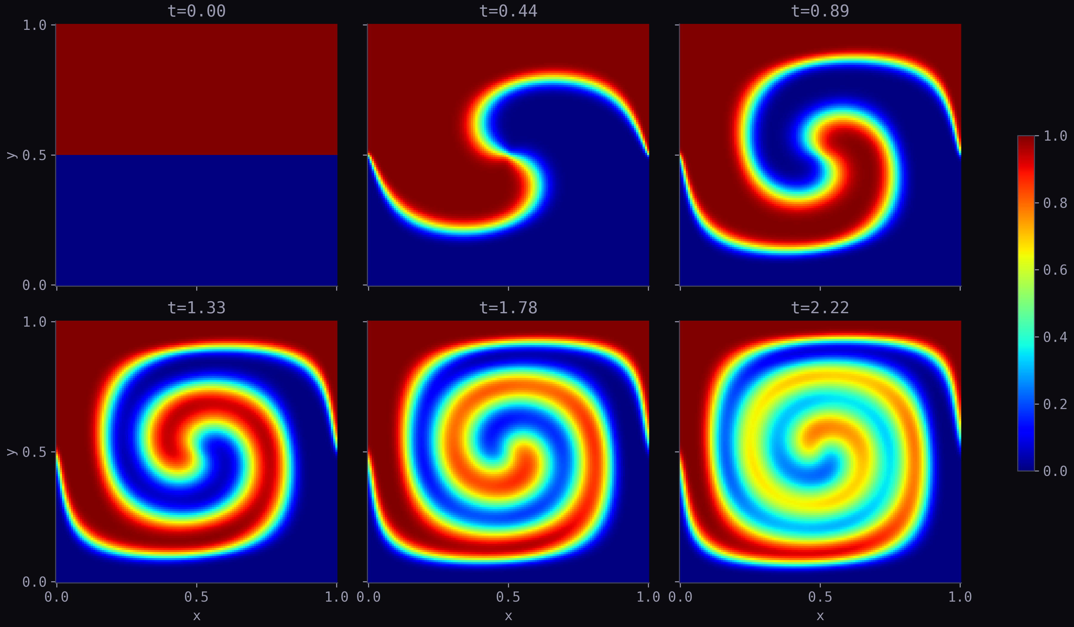
Diffusivity $D(u) = u^n$ vanishes where $u=0$, producing finite-speed propagation and sharp fronts — a hallmark of nonlinear degenerate diffusion. BDF handles the resulting stiffness.

Example 02

Advection/Diffusion in 2D

$$q_t = -\mathbf{u} \cdot \nabla q + k\nabla^2 q$$

$u = \pi\psi_0\sin^2(\pi x)\sin(2\pi y)$

$v = -\pi\psi_0\sin(2\pi x)\sin^2(\pi y)$

Advection of a scalar by a divergence-free vortex velocity field (Taylor–Green vortex).

1Define

nx, ny = 64, 64
x = np.linspace(0, 1, nx); y = np.linspace(0, 1, ny)
u = lambda x,y: np.sin(np.pi*x)**2 * np.sin(2*np.pi*y)
v = lambda x,y: -np.sin(2*np.pi*x) * np.sin(np.pi*y)**2
eq = PDE('T', x=x, y=y)
eq.add_advection(velocity_x=u, velocity_y=v)
eq.add_diffusion(diffusivity=1e-4)

2Constrain

T0 = np.zeros((nx, ny)); T0[:, nx//2:] = 1.0
eq.set_ic(T0)
eq.set_bc(side='all', kind='neumann', value=0.0)

3Solve

sol = eq.solve(t_span=(0, 4))

2D · Vortex advection · 6 snapshots

Figure: 6-panel time evolution

Replace with your matplotlib output

Example 03

Coupled Reaction-Diffusion A + B → C

$\dfrac{\partial c_A}{\partial t} = D_A \dfrac{\partial^2 c_A}{\partial x^2} - k_1 c_A c_B$

$\dfrac{\partial c_B}{\partial t} = D_B \dfrac{\partial^2 c_B}{\partial x^2} - k_1 c_A c_B$

$\dfrac{\partial c_C}{\partial t} = D_C \dfrac{\partial^2 c_C}{\partial x^2} + k_1 c_A c_B$

1Define

DA, DB, DC = 20e-4, 10e-4, 5e-4; k1 = 100.0
def src_AB(x, cA, cB, cC): return -k1 * cA * cB
def src_C (x, cA, cB, cC): return +k1 * cA * cB
eqA = PDE('cA', x=x); eqA.add_diffusion(DA); eqA.add_source(src_AB)
eqB = PDE('cB', x=x); eqB.add_diffusion(DB); eqB.add_source(src_AB)
eqC = PDE('cC', x=x); eqC.add_diffusion(DC); eqC.add_source(src_C)

2Constrain

eqA.set_ic(gaussian(x)); eqB.set_ic(1.0); eqC.set_ic(0.0)
eqA.set_bc(side=['left','right'], kind='dirichlet', value=[5.0,0.0])
eqB.set_bc(side=['left','right'], kind='dirichlet', value=[0.0,3.0])

3Solve

sys = PDESystem([eqA, eqB, eqC])
sol = sys.solve(t_span=(0, 100), method='BDF')

3-field coupled system · PDESystem

Figure: IC → steady-state profiles

Replace with your matplotlib output

Example 04

Stokes' Second Problem — time-dependent BC

$$u_t = \nu \, u_{xx}$$

Oscillating wall: $U_\text{plate}(t) = A\cos(\omega t)$

1Define

eq = PDE('u', y)
eq.add_diffusion(diffusivity=nu)

2Constrain

eq.set_bc(side='left', kind='dirichlet',
          value=lambda t: U0 * np.cos(omega * t))
eq.set_bc(side='right', kind='dirichlet', value=0.0)
eq.set_ic(0.0)

3Solve

T = 2*np.pi / omega   # one period
sol = eq.solve(t_span=(0, 4*T), method='BDF')

Analytical solution:

$u(y,t) = A\,e^{-\delta y}\cos(\omega t - \delta y)$, $\delta = \sqrt{\omega/2\nu}$

Time-dependent BC · 1D diffusion

Figure: velocity profile vs. depth

Replace with your matplotlib output

Example 05

Potential Flow over a Cylinder

$$\nabla^2\psi = 0$$

Stream-function formulation. Cylinder enforced as an interior Dirichlet constraint ($\psi = y_c$ on cylinder surface).

1Define

eq = PDE('psi', x=x, y=y)
eq.add_diffusion(diffusivity=1.0)

2Constrain

cylinder = (X-cx)**2 + (Y-cy)**2 <= R**2
eq.set_bc(side=['bottom','top'], kind='dirichlet', value=[0.0,3.0])
eq.set_bc(side=['left','right'], kind='neumann',   value=0.0)
eq.set_interior_bc(mask=cylinder, kind='dirichlet', value=cy)
eq.set_ic(0)

3Solve

sol = eq.solve_steady()

Velocity recovered as: $u = \partial\psi/\partial y$, $v = -\partial\psi/\partial x$

Steady-state · Interior BC · Streamlines

Figure: Flow over cylinder

Figure: uPDE logo flow

Example 06

Darcy Flow — Heterogeneous Porous Medium

$$\nabla \cdot \left[K(\mathbf{x})\,\nabla p\right] = 0$$

Log-normal random permeability field. High-contrast $K$ produces channeling and preferential flow paths.

1Define

# random log-normal permeability
log_K = gaussian_filter(np.random.randn(nx,ny), sigma=12)
K     = np.exp(3 * log_K / log_K.std())
eq = PDE('p', x=x, y=y)
eq.add_diffusion(diffusivity=K)

2Constrain

eq.set_bc(side='all',              kind='neumann',   value=0.0)
eq.set_bc(side=['left','right'], kind='dirichlet', value=[1.0, 0.0])

3Solve

sol = eq.solve_steady()

Steady-state · Spatially-varying K · 200×200

Figure: log₁₀K permeability field

Figure: Darcy flux |q| = K|∇p|

Figure: Pressure + streamlines

Example 07

Electric Potential — Lossy Dielectric

$$\nabla \cdot (\varepsilon_c \nabla V) = 0, \quad \varepsilon_c = \varepsilon_r + j\varepsilon_i$$

$\nabla \cdot (\varepsilon_r\nabla V_r) - \nabla \cdot (\varepsilon_i\nabla V_i) = 0$

$\nabla \cdot (\varepsilon_r\nabla V_i) + \nabla \cdot (\varepsilon_i\nabla V_r) = 0$

Split into coupled real/imaginary PDEs. The U logo acts as a lossy dielectric inclusion ($\varepsilon_c = 1.5 - 3j$).

1Define

eq_r = PDE("Vr", x=x, y=y)
eq_r.add_diffusion(diffusivity=eps_r)
eq_r.add_term(lambda Vi, Div_flux_x, Div_flux_y:
  -Div_flux_x(eps_i,Vi) - Div_flux_y(eps_i,Vi))

eq_i = PDE("Vi", x=x, y=y)
eq_i.add_diffusion(diffusivity=eps_r)
eq_i.add_term(lambda Vr, Div_flux_x, Div_flux_y:
   Div_flux_x(eps_i,Vr) + Div_flux_y(eps_i,Vr))

3Solve

sol = PDESystem([eq_r, eq_i]).solve_steady(method="linear")

Coupled · Complex permittivity · The Potential of the U

Figure: Electric field intensity |E| [V/m]

Replace with your matplotlib output

Example 08

Combustion — Mixture Fraction & Flamelet Chemistry

$$\frac{\partial Z}{\partial t} + u(y)\frac{\partial Z}{\partial x} = D\nabla^2 Z$$

Dedicated MixtureFraction equation factory. Tabulated flamelet chemistry via Burke–Schumann or Cantera.

1Define

from upde import MixtureFraction
eq = MixtureFraction('Z', x=x, y=y,
  velocity_x=u_field, velocity_y=0.0, diffusivity=D)

2Constrain

eq.set_bc(mask=jet_mask_left,    kind='dirichlet', value=1.0) # fuel
eq.set_bc(mask=coflow_mask_left, kind='dirichlet', value=0.0) # air
eq.set_bc(side='right',         kind='neumann',   value=0.0)
eq.set_ic(0.0)

3Solve + post-process

sol = eq.solve(t_span=(0, 20))
table = FlameletTable.burke_schumann(Z_st=0.055, ...)
T_final   = table.T(sol.Z[:,:,-1])
Y_CH4     = table.Y('CH4', sol.Z[:,:,-1])

MixtureFraction · FlameletTable · Burke–Schumann

Figure: Temperature [K]

Figure: CH₄ mass fraction

Figure: O₂ / CO₂ mass fractions

Example 09

Wave Equation — 2D Gaussian Pulse

$$u_{tt} = c^2\nabla^2 u$$

Reduced to first-order system:

$\dfrac{\partial u}{\partial t} = u^t, \qquad \dfrac{\partial u^t}{\partial t} = c^2\nabla^2 u$

1Define

from upde import WaveEquation
weq = WaveEquation('u', 'ut', x=x, y=y, speed=1.0)

2Constrain

u0 = np.exp(-((X-cx)**2 + (Y-cy)**2) / (2*sig**2))
weq.u.set_ic(u0);  weq.ut.set_ic(0.0)
# reflecting walls
weq.u.set_bc( side='all', kind='dirichlet', value=0.0)
weq.ut.set_bc(side='all', kind='dirichlet', value=0.0)

3Solve

sol = weq.solve(t_span=(0, 3))

WaveEquation factory · Dirichlet walls · 12 snapshots

Figure: 12-panel pulse evolution in square cavity

Replace with your matplotlib output

Example 10

Navier-Stokes — Flow over a Cylinder

$\dfrac{\partial u}{\partial t} + u\dfrac{\partial u}{\partial x} + v\dfrac{\partial u}{\partial y} = -\dfrac{1}{\rho}\dfrac{\partial p}{\partial x} + \nu\left(\dfrac{\partial^2 u}{\partial x^2}+\dfrac{\partial^2 u}{\partial y^2}\right)$

$\dfrac{\partial v}{\partial t} + u\dfrac{\partial v}{\partial x} + v\dfrac{\partial v}{\partial y} = -\dfrac{1}{\rho}\dfrac{\partial p}{\partial y} + \nu\left(\dfrac{\partial^2 v}{\partial x^2}+\dfrac{\partial^2 v}{\partial y^2}\right)$

$\dfrac{\partial p}{\partial t} = -\beta\left(\dfrac{\partial u}{\partial x}+\dfrac{\partial v}{\partial y}\right) + \varepsilon\nabla^2 p$

Artificial compressibility method. Pressure equation drives divergence to zero.

1Define

from upde import NavierStokes2D
ns = NavierStokes2D('u','v','p', x=x, y=y,
                    nu=0.01, rho=1.0, beta=0.7)

2Constrain

ns.u.set_bc(side=['bottom','top'], kind='dirichlet', value=0.0)
ns.u.set_bc(side='left',            kind='dirichlet', value=1.3)
mask = (x[:,None]-cx)**2 + (y[None,:]-cy)**2 <= 0.5**2
ns.u.set_interior_bc(mask=mask, kind='dirichlet', value=0.0)
ns.v.set_interior_bc(mask=mask, kind='dirichlet', value=0.0)

3Solve

sol = ns.solve(t_span=(0, 10))

NavierStokes2D · Artificial compressibility · Re≈65

Figure: Velocity magnitude + streamlines

Figure: Von Kármán wake behind cylinder